I’ve been working on base cartography for the research area in Rwanda. Unlike here in Cleveland, we have some great topography to work with, so we can leverage that for basemaps. But, it’s such a beautiful landscape, I didn’t want to sell these hillshades short by doing a halfway job, so I’ve been diving deep.
Background
First, some legacy. I read three great blog posts on hillshades. One was from ESRI revealing their “Next Generation Hillshade”. Drawing on Swiss Cartographic Traditions, these are some nice looking hillshades using lighting sources from multiple directions (more on this later):

Next, we look to Peter Richardsons’s recent post on Mapzen’s blog regarding terrain simplification.

I tried (not nearly as hard as I should have) to understand their code, when I saw a link to Daniel Huffman’s blog post from 2011 on terrain generalization: On Generalization Blending for Shaded Relief.

That’s when I saw the equation:
((Generalized DEM * Weight) + (Detailed DEM * (WeightMax – Weight))) / WeightMax
I’ll let you read these posts, rather than rehashing, but here’s what I did toward adding to them. The gist of Daniel and Peter’s approach is to blend together a high resolution and lower resolution version of the DEM based on a weighting factor. Both use a standard deviation filter to determine where to use the high resolution DEM vs resampled version — if the location is much higher or lower than it’s neighbors, it is considered an important feature, and given detail, otherwise the low resolution version is used (actually, I suspect Mapzen’s approach is only highlighting top features based on their diagrams, but I haven’t dived into the code to verify).
The Need
Excuse the colors, we’ll fix those at the end, but this allows us to simplify something that looks like this:

Into something that looks like this:

See how the hilltops and valleys remain in place and at full detail, but some of the minor facets of the hillsides are simplified? This is our aim.
I developed a pure GDAL approach for the simplification. It is purely command line, has hardcoded file names, etc, but could be done with a python or other API and turned into a proper function. TL:DR: this is not yet refined but quite effective.
Landscape Position
If you’ve been following my blog for a while, you may recall a series of blog posts on determining landscape position using gdal.
This, with small modification, is a perfect tool for determining where to retain DEM features and where to generalize. The one modification is to calculate standard deviation from our simple difference data.
The Tools
Generalization
This file contains hidden or bidirectional Unicode text that may be interpreted or compiled differently than what appears below. To review, open the file in an editor that reveals hidden Unicode characters.
Learn more about bidirectional Unicode characters
| # Documented at http://wp.me/phWh4-10l | |
| # First we fill holes in the DEM: | |
| gdal_fillnodata dem30.img dem30_fill.tif | |
| # Now we are going to create a blurred version of the DEM. We'll use this as the generalized DEM | |
| # in our blended DEM | |
| gdalwarp -tr 400 400 -r lanczos -co "BLOCKXSIZE=512" -co "BLOCKYSIZE=512" dem30_fill.tif dem30_400.tif | |
| gdalwarp -tr 30.929927379942203 30.929927379942203 -r lanczos -co "BLOCKXSIZE=512" -co "BLOCKYSIZE=512" dem30_400.tif dem30_400-30.tif | |
| # We also need a more generalized DEM to for our TPI work. | |
| # See https://smathermather.com/category/ecology/landscape-position/ for more info | |
| gdalwarp -tr 5000 5000 -r lanczos dem30_fill.tif dem30_5000.tif | |
| gdalwarp -tr 30.929927379942203 30.929927379942203 -r lanczos dem30_5000.tif dem30_5000-30.tif | |
| # To avoid issues with differently sized images when we use gdal_calc, we'll stack our images into a single image | |
| gdal_merge -separate -of GTiff -o tpistack.tif dem30_5000-30.tif dem30_fill.tif | |
| # Now we calculate a normalized TPI (effectively calculating Standard Deviation over 5000 meter radius) | |
| gdal_calc -A tpistack.tif -B tpistack.tif –A_band=1 –B_band=2 –outfile=tpi.tif –calc="sqrt((B * 1.00000 – A * 1.00000) * (B * 1.00000 – A * 1.00000))" | |
| # Same trick here — we stack our different images to ensure we have our image dimensions equal | |
| # for gdal_calc | |
| gdal_merge -separate -of GTiff -o stack.tif tpi.tif dem30_400-30.tif dem30_fill.tif | |
| # And now we calculate our weighted DEM | |
| gdal_calc -A stack.tif -B stack.tif -C stack.tif –A_band=2 –B_band=1 –C_band=3 –outfile=result.tif –calc="((A * B) + (C * (288 – B))) / 288" | |
| # We'll convert this to a PNG for use in Povray. See https://gist.github.com/smathermather/cd610cf0b930cbbba61d341c6ababfd8 | |
| gdal_translate -ot UInt16 -of PNG result.tif pov-viewshed\result.png | |
Back to those ugly colors on my hillshade version of the map. They go deeper than just color choice — it’s hard not to get a metallic look to digital hillshades. We see it in ESRI’s venerable map and in Mapbox’s Outdoor style. Mapzen may have avoided it by muting the multiple-light approach that ESRI lauds and Mapbox uses — I’m not sure.
HDRI (Shading)
To avoid this with our process (HT Brandon Garmin) I am using HDRI environment mapping for my lighting scheme. This allows for more complicated and realistic lighting that is pleasing to the eye and easy to interpret. Anyone who has followed me for long enough knows where this is going: straight to Pov-Ray… :
This file contains hidden or bidirectional Unicode text that may be interpreted or compiled differently than what appears below. To review, open the file in an editor that reveals hidden Unicode characters.
Learn more about bidirectional Unicode characters
| #include "shapes.inc" | |
| #include "colors.inc" | |
| #include "textures.inc" | |
| // Dropped in from http://wiki.povray.org/content/HowTo:Use_radiosity | |
| #local p_start = 64/image_width; | |
| #local p_end_tune = 8/image_width; | |
| #local p_end_final = 4/image_width; | |
| #local smooth_eb = 0.50; | |
| #local smooth_count = 75; | |
| #local final_eb = 0.1875; | |
| #local final_count = smooth_count * smooth_eb * smooth_eb / (final_eb * final_eb); | |
| global_settings{ | |
| radiosity | |
| { | |
| pretrace_start p_start // Use a pretrace_end value close to what you | |
| pretrace_end p_end_tune // intend to use for your final trace | |
| count final_count // as calculated above | |
| nearest_count 10 // 10 will be ok for now | |
| error_bound final_eb // from what we determined before, defined above | |
| // halfway between 0.25 and 0.5 | |
| recursion_limit 2 // Recursion should be near what you want it to be | |
| // If you aren't sure, start with 3 or 4 | |
| } | |
| } | |
| // Orthographic camera allows us to return non-perspective image of elevation model | |
| camera { | |
| orthographic | |
| location <0.5, 2, 0.75> | |
| look_at <0.5,0,0.75> | |
| right 0.25*x // horizontal size of view — I have this zoomed in on my area of interest. | |
| up 0.25*y // vertical size of view — set to 1*x and 1*y to get full DEM hillshade returned | |
| } | |
| // Here's where the height field get's loaded in for shading | |
| height_field { | |
| png "result.png" | |
| water_level 0.0 | |
| smooth | |
| texture { | |
| pigment { | |
| rgb <1, 1, 1> | |
| } | |
| } | |
| finish { | |
| ambient 0.2 | |
| diffuse 0.8 | |
| specular 0 | |
| roughness 40 | |
| } | |
| scale <1, 1, 1> | |
| translate <0,0,0> | |
| } | |
| // Pulled in from http://www.f-lohmueller.de/pov_tut/backgrnd/p_sky10.htm | |
| // Using an HDR from http://www.pauldebevec.com/Probes/ | |
| sky_sphere{ | |
| pigment{ | |
| image_map{ hdr "rnl_probe.hdr" | |
| gamma 0.25 | |
| map_type 1 interpolate 2} | |
| }// end pigment | |
| rotate <0,40,0> // | |
| } // end sphere with hdr image ———– | |
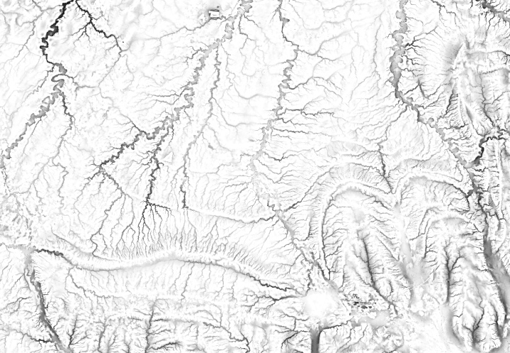
Results
The results? Stunning (am I allowed to say that?):


The color is very simple here, as we’ll be overlaying data. Please stay tuned.
