The last two days, I have been working with Olivier Jean Leonce Manzi here at Karisoke Research Center on the question of the relationship between gorilla food plants biomass and the ranging patterns of gorillas outside Volcanoes National Park (VNP) in Rwanda.

Even though Volcanoes National Park is set aside and gorillas thrive inside, they don’t strictly stay within the bounds of the park — often leaving the park to forage in the adjacent farming communities. This tendency is an opportunity for human / wildlife conflict, and thus it is important to understand the relationship between gorilla browsing habits outside the park and their food resources in these farming communities.
Among the food plants in the study, eucalyptus, a non-native, is planted widely in Rwanda as a fast growing timber source. Gorillas like to climb up eucalyptus, stripping the outer bark, and use their teeth to scrape the inner bark from the tree. For larger trees, this seems to have little effect. For smaller trees, it can kill the tree easily, either by the weight of the gorilla on the tree or the damage to the vascular system of the tree.

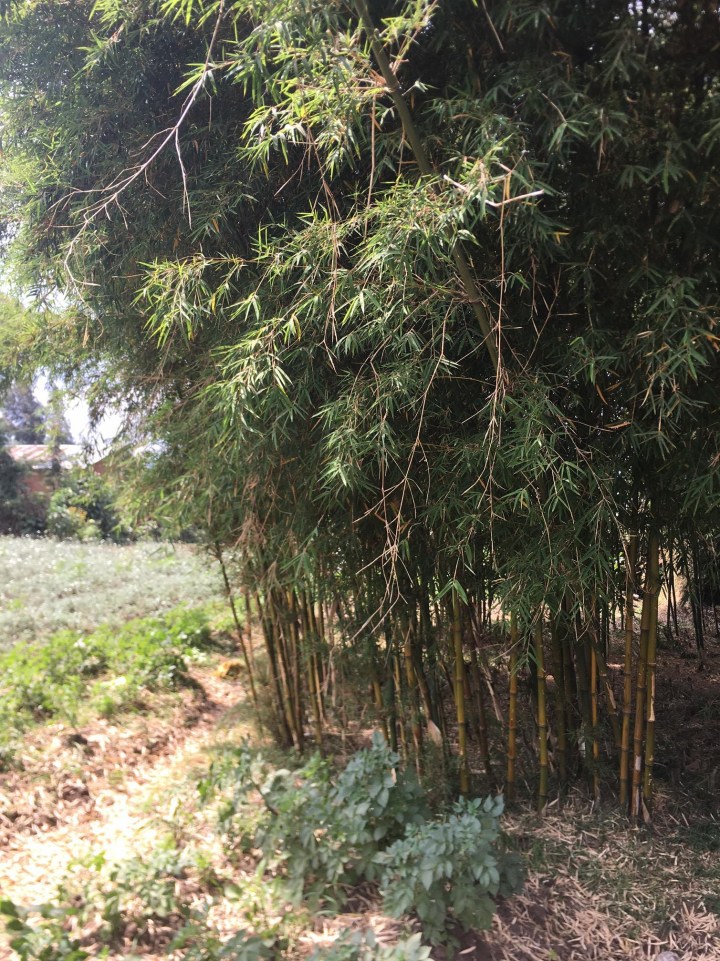
Bamboo, native to the region, is widely planted outside VNP (and grows in forests inside VNP). As it sprouts during rainy season, it is a favorite food of gorillas both inside and outside the park.
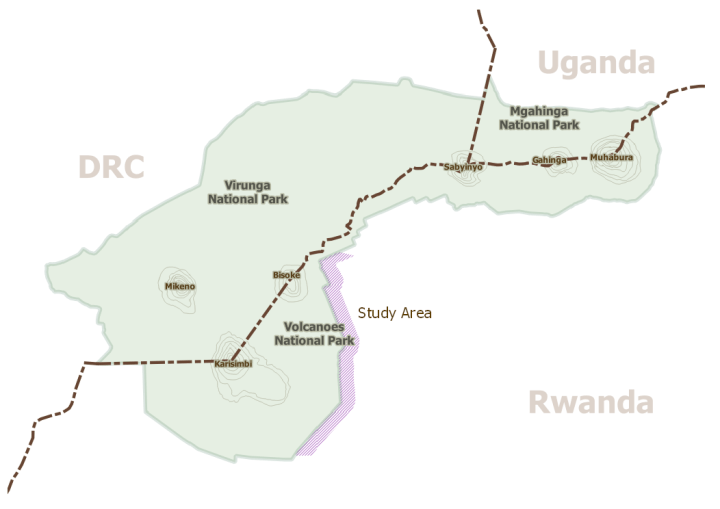
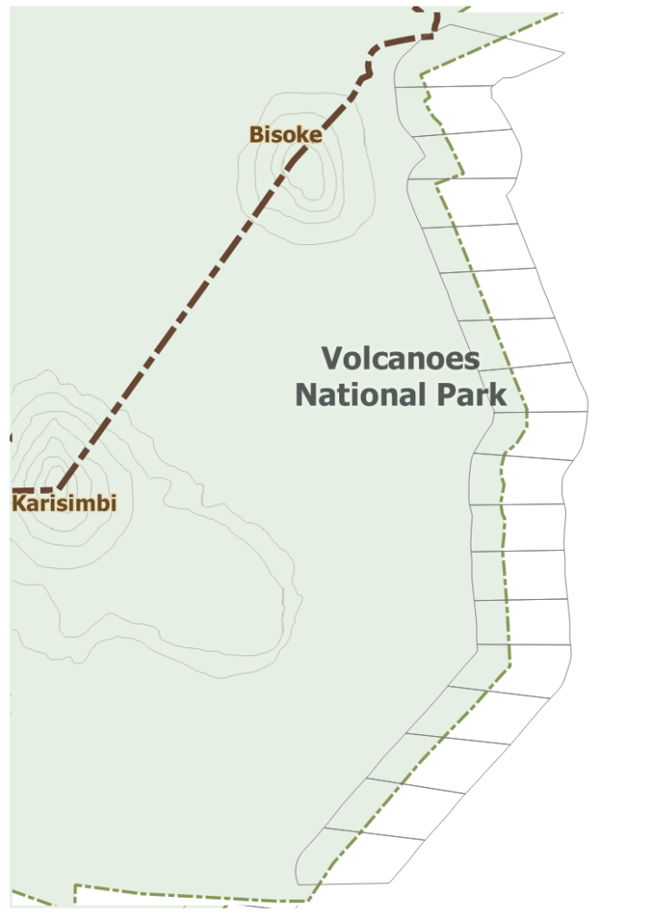
Olivier’s study area is in the farming area along the base of Karisimbi and Bisoke Volcanoes just outside VNP. (Quick aside: it was a combination of Karisimbi and Bisoke names that formed Karisoke Research Center’s name).
The two datasets we want to compare for the study are counts of gorillas ranging outside the park and transects of gorilla plant food biomass, also outside the park.


The measurements that Olivier made on gorilla plant food biomass is that of herbs (overall), trees (overall), eucalyptus, bamboo, and rubus (a group commonly known as raspberries, blackberries, dewberries, etc.) — favored foods for gorillas especially outside the park.

For the purposes of analysis, Olivier grouped the vegetation plots and gorilla counts into 18 approximately equal zones. Gorilla counts and vegetation plots were summarized per zone and compared.
I remember his project as one of the more difficult ones to wrap my head around when I was here in December. In summary, here’s the problem that we wanted to solve: given a dataset of gorilla food biomass outside the park, and counts of gorillas outside the park, can we establish a relationship between the two. It should be an easy problem: on one side of the equation, we have count data, on the other ratio data. My first thought would be to apply a Poisson approach.
Gorilla.count ~ Herbs.biomass + Tree.biomass + Eucalyptus.biomass + Bamboo.biomass + Rubus.biomass
But we quickly run into a problem: our data are not independent in time or in space, and so a simple Poisson approach is likely not appropriate.
For as much work as I’ve done in the geospatial space, I have done precious little with spatial statistics, so this posed a conundrum to me. I can’t remember now if it was through much googling, or the great stewardship of Dr. Patrick Lorch, the research manager at my institution, that we settled upon using a Markov chain Monte Carlo (MCMC) approach to the problem. The advantage to this approach is that we can do the analysis using a Poisson distribution without regard to autocorrelation. In the R statistical package, this is an easy analysis to set up.
This file contains hidden or bidirectional Unicode text that may be interpreted or compiled differently than what appears below. To review, open the file in an editor that reveals hidden Unicode characters.
Learn more about bidirectional Unicode characters
| — | |
| title: "gorilla_plant_biomass" | |
| author: "Olivier Jean Leonce Manzi and Stephen Vincent Mather" | |
| date: "July 3, 2017" | |
| output: html_document | |
| — | |
| “`{r setup, include=FALSE} | |
| knitr::opts_chunk$set(echo = TRUE) | |
| “` | |
| ## R Markdown | |
| “`{r code, echo=FALSE} | |
| library(mcmc) | |
| zones <- | |
| read.csv("zones_with_biomass.csv") | |
| out <- glm(Gorillas.counts ~ Herbs.biomass..g.m2. + Trees.biomass..stems.m2. + Eucalyptus.biomass..stems.m2. + Bamboos.biomass..stems.m2. + Rubus.biomass..g.m2., family = poisson, data = zones) | |
| summary(out) | |
| “` |
Finally, we’ll close with a picture of Olivier working on his literature review for the methods section:


I don’t think the MCMC was my idea, so thanks to Google. I am working on some ways to look at the spatial autorrelation by plotting the residuals against the distance between Gorilla sightings (a kind of correlogram, I think). This shows how big a problem autocorrelation is. Then we can try including model terms for the autocorrelation into the glm, and then look again at the residual plot to see if the pattern in the residuals is reduced.