Much like the early days of GPS/GNSS, the longer we have drones in the air, the more capacity we build and layer upon previous work. To that end, a colleague of mine has a request to gather video and stills over an area slated for possible installation of a zip line. The request includes flying the path of future zipline. I had concerns whether we can safely fly that path: it is winter here in Ohio, hampering our drones detect and avoid sensors due to leaf-off condition on the trees.

Enter old data

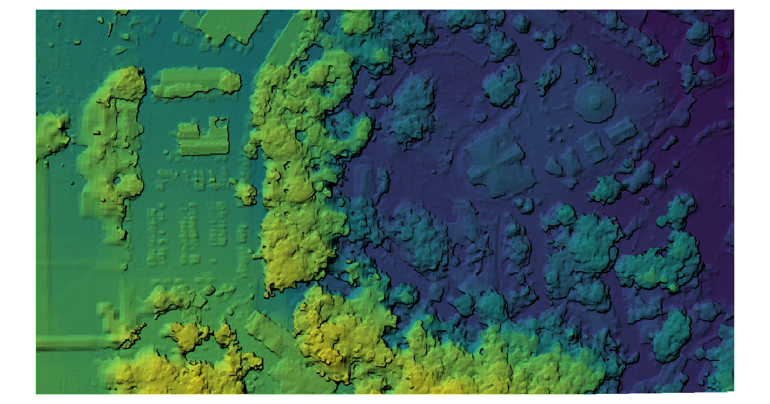
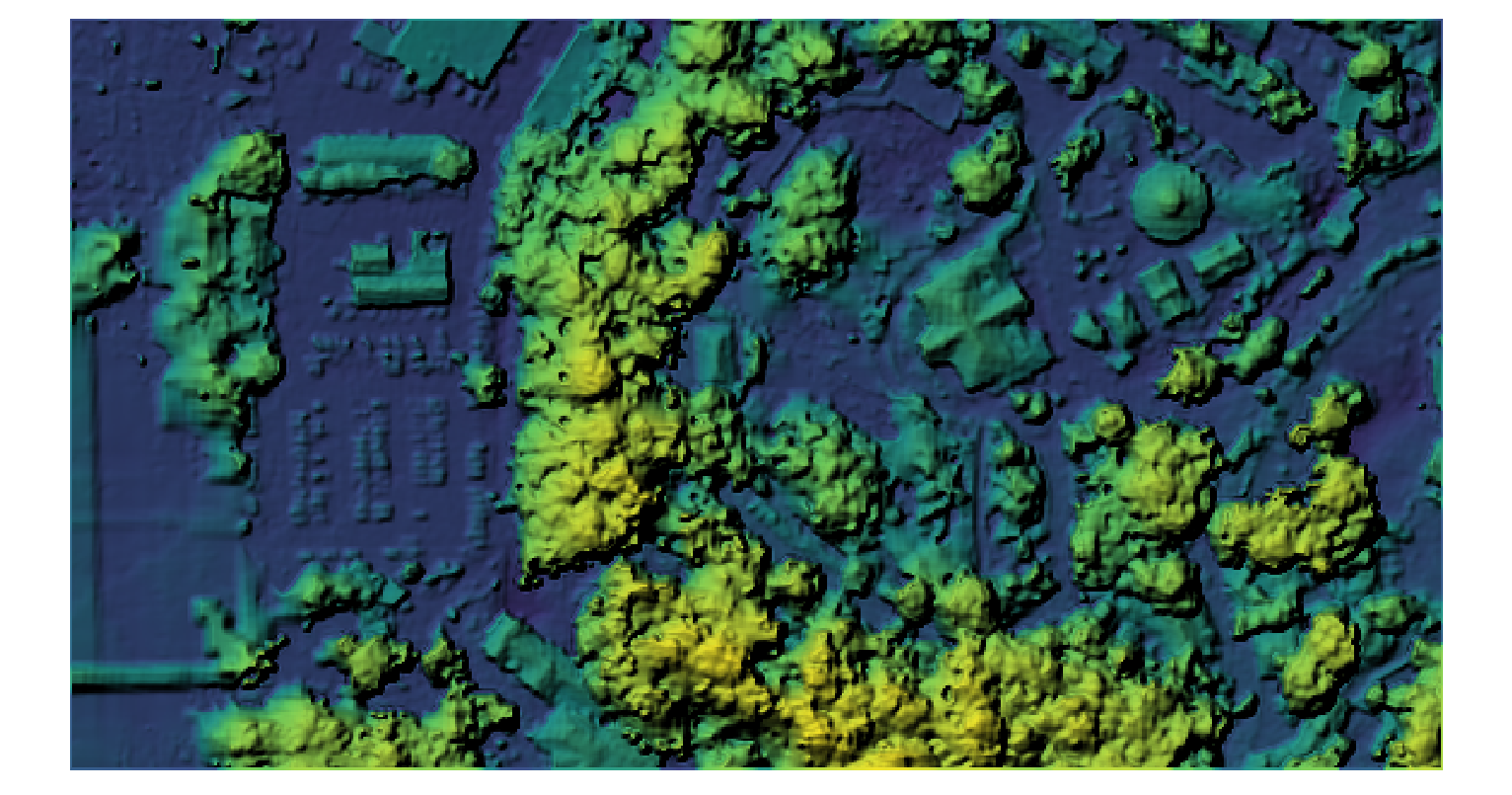
This location we flew early in the Autumn of 2016, so we have a full digital surface model for the location. As trees have undoubtedly grown the last 4 years, we need to take any heights as approximate, but it is a useful starting place for sanity checking out flight plan. The location is, not surprisingly, a steep slope, that as is common in Northeast Ohio is lousy with lovely mature forest.

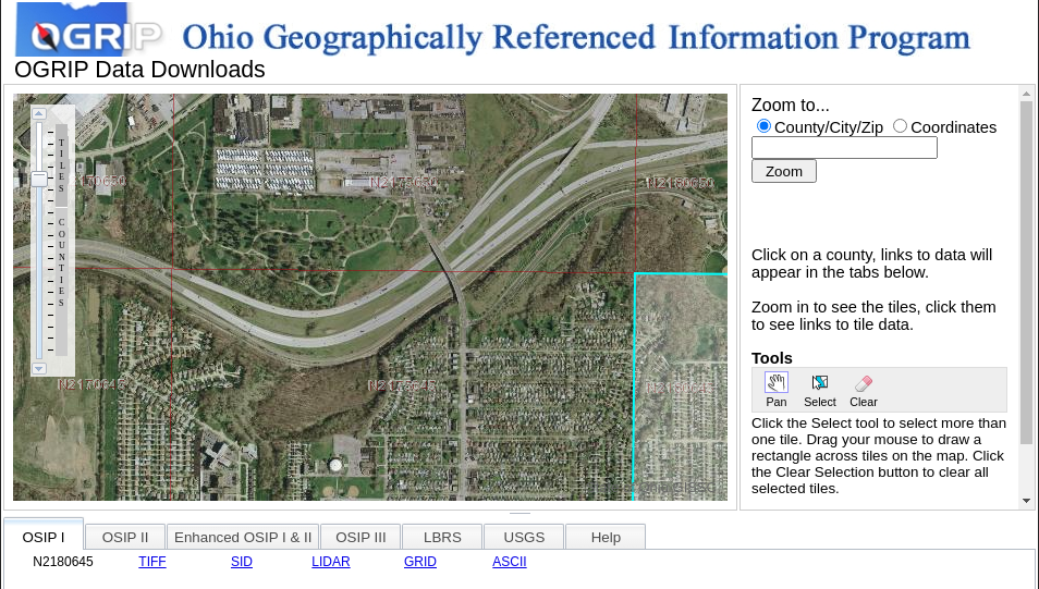
As the first stage in estimating our risk, we will generate a digital height model from digital surface and terrain models. As the 2016 flights were not executed with high levels of overlap, we can assume that the DTM from OpenDroneMap won’t be adequate, so we’ll seek an alternative source. Our county elevation models are quite good, but the State of Ohio’s Statewide Imagery Program LiDAR derived elevation models will serve our purpose. We’ll download from the ASCII link, and rename the resulting txt file with a *.asc extension to prompt QGIS to recognize the file format.

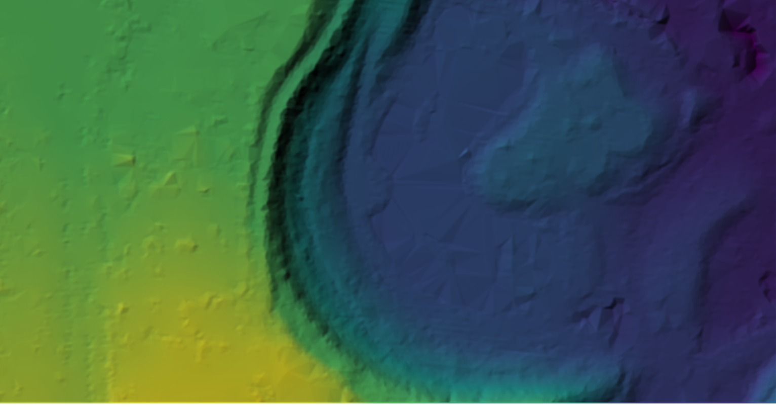
We can style the elevation data in QGIS for visualization. Aside from some noise, and lack of flat-water postprocessing, the data look reasonable.

Downloading data from WebODM is straightforward: click anywhere on the map and a list of downloadable assets appears. We will download the “Terrain Model” and visualize similarly in QGIS:

What’s the difference?

I recommend ensuring coordinate systems, elevation scale, etc. are all the same between elevation models being prepped for differencing, and that the area is subset to approximately the area of interest.

Coordinate system and subsetting

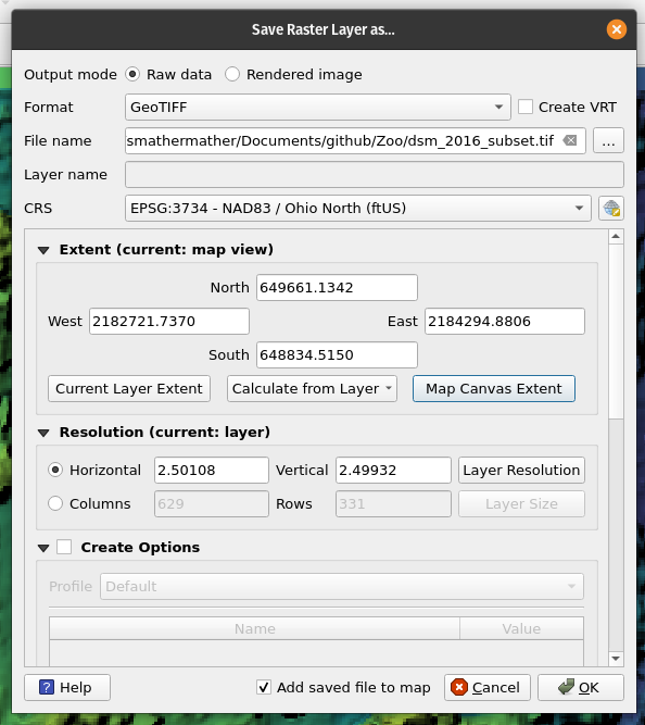
I usually take the easy way out in accomplishing this by using “Save Raster Layer as…” in QGIS, choose “Map Canvas Extent” as the output extent, and choose the appropriate Coordinate Reference System, in our case EPSG:3734.

Now that both rasters are in the same CRS and the same focus area, we need to ensure that they match vertical scales. As the 2016 data was shot with a commodity GPS and commodity camera, we can expect some small bias in our scale, and elevations in OpenDroneMap default to meters, while our engineers and drone pilots usually work in feet.

Scratching the itch

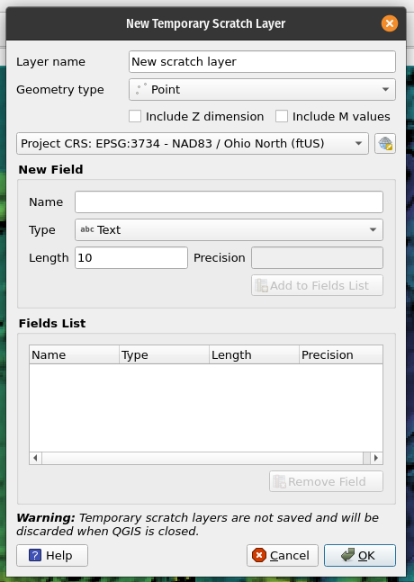
We will create a scratch layer and digitize a few points in open areas where we anticipate the terrain and surface models should be the same, careful to distribute the points across the study area horizontally and vertically.

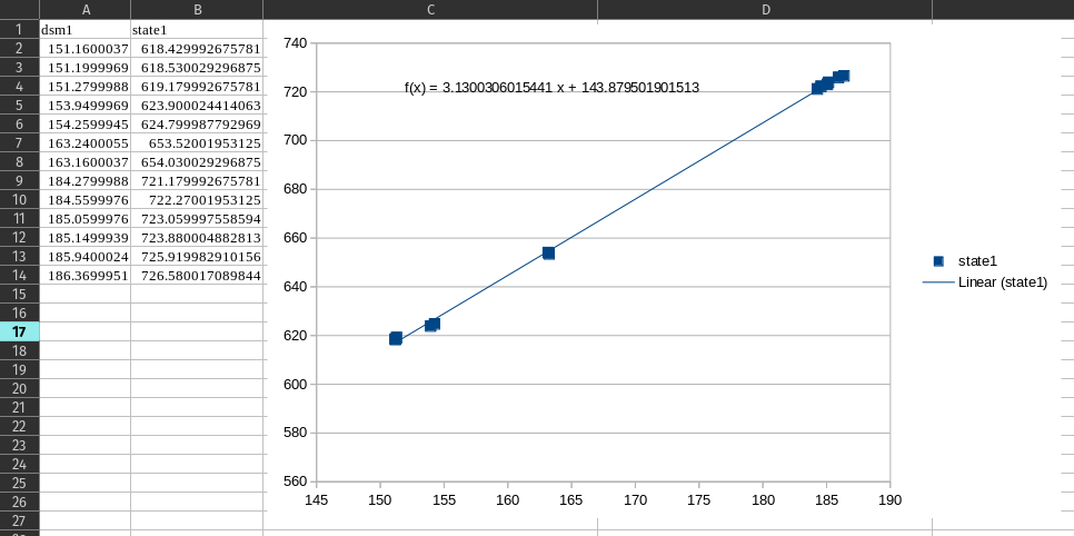
After digitizing our points, we can extract the raster values at these points and derive an equation to convert between elevation values. We will use Processing Toolbox: “Sample Raster Values” to extract the values and compare. Under most circumstances, a simple linear regression will tell us how to convert between the two. We would expect the scale factor to be close to a meters/feet conversion, or ~3.28. As expected for the commodity GPS and camera, we have a small 5% difference from this in our scaling factor, but it is close enough for our purposes.

Making the difference

If we want to avoid certain artifacts of calculations across pixel sizes, we might take one more step in GDAL and resample to a common pixel size using GDAL, though this won’t affect our analysis much:

gdalwarp -r lanczos -tr 2.5 2.5 dsm_2016_subset_stateplane.tif dsm_2016_subset_stateplane_2.5.tif

We now have all of our conversions in place and can safely calculate our differences using “Raster Calculator” using a Raster Calculator Expression similar to the following which performs our scaling, offset, and difference in a single step:

("dsm_2016_subset_stateplane_2.5@1" * 3.13 + 143.8795) - "dtm@1"

Bring it home

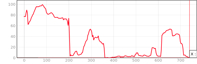
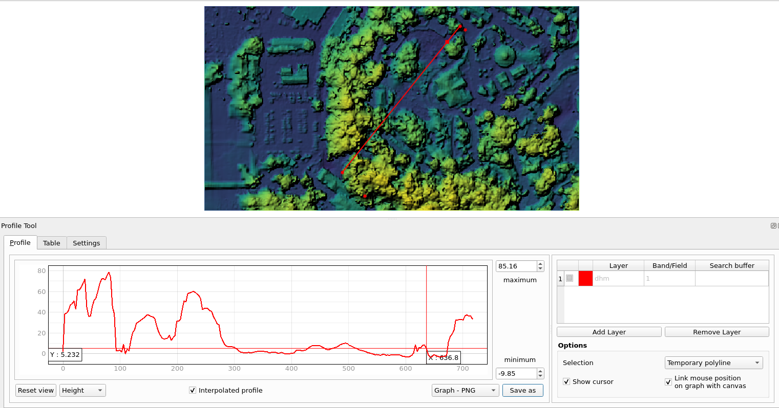
Using QGIS “Terrain Profile” plugin, we can now plot our tree heights above ground and have a sense of what heights are safe for our linear paths here. One could also load the DSM into flight planning software and optimize for other flight types, but that’s another blog post entirely.